PEtab data format specification 2.0

Warning

This document is a draft and subject to change.

Format version: 2.0.0

This document explains the PEtab data format.

Purpose

PEtab provides a standardized framework for defining parameter estimation problems in systems biology, particularly for Ordinary Differential Equation (ODE) models.

Scope

The scope of PEtab is the complete specification of parameter estimation problems in typical systems biology applications. In practise, data-driven modeling often begins with either (i) a computational model of a biological system that requires calibration or (ii) experimental data that need integration and analysis through a computational model.

Measurements are linked to the biological model by an observation and noise model. Often, measurements are taken after some experimental perturbations have been applied, which are represented as derivations from a generic model (Figure 1A). Therefore, one goal was to specify such a setup in the least redundant way. Furthermore, we wanted to establish an intuitive, modular, machine- and human-readable and -writable format that makes use of existing standards.

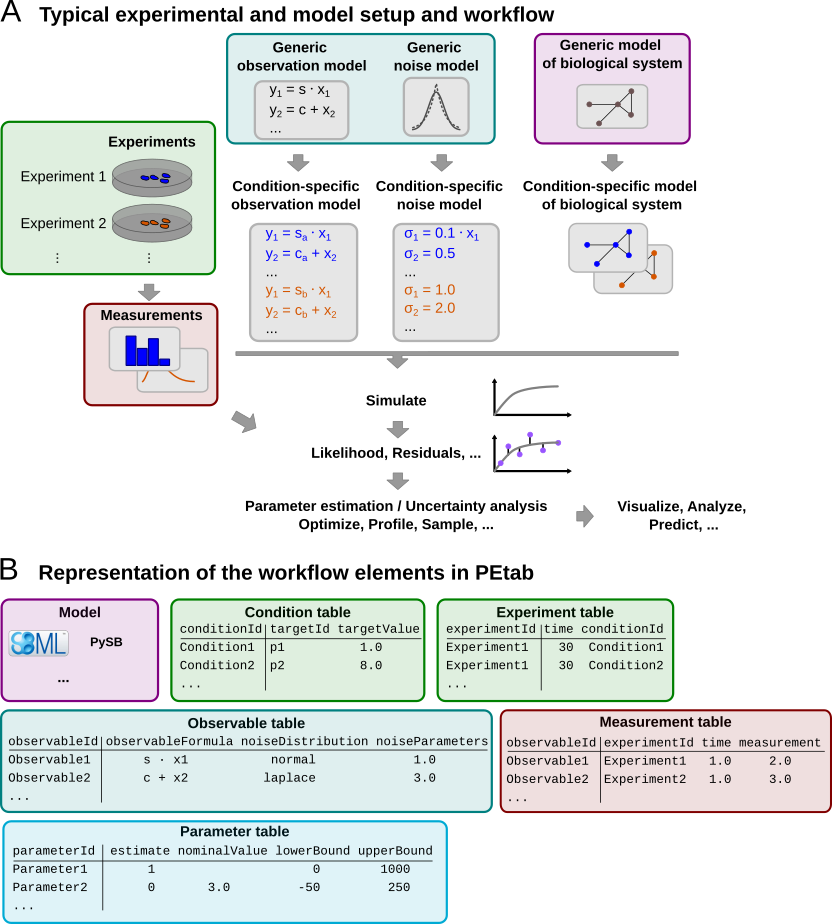
**Figure 1: A typical setup for data-based modeling studies and its representation in PEtab.**

Overview

The PEtab data format defines a parameter estimation problem using multiple text-based files in YAML and Tab-Separated Values (TSV) format (Figure 2), including:

A grouping file that lists all of the following files and provides additional information including extensions [YAML].
Parameter file(s) to set parameter values globally, and to specify the parameters to be estimated as well as their parameter bounds and prior distributions [TSV].
Model file(s) specifying the base model(s) [SBML, CELLML, BNGL, PYSB, …].
Observable file(s) defining the observation model [TSV].
Measurement file(s) containing experimental data used for model fitting [TSV].
(optional) Condition file(s) specifying model inputs and condition-specific parameters [TSV].
(optional) Experiment file(s) describing sequences of experimental conditions applied to the model [TSV].
(optional) Mapping file(s) assigning PEtab-compatible IDs to model entities that do not have valid PEtab IDs themselves, and providing additional annotations [TSV].

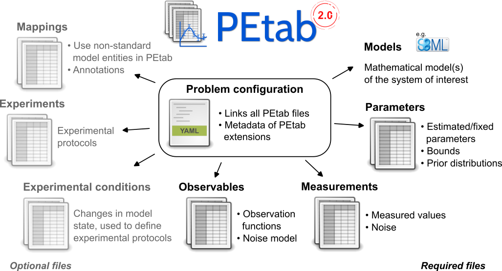
**Figure 2: Files constituting a PEtab problem.**

Figure 1B shows how those files relate to a typical data-based modeling setup.

The following sections outline the minimum requirements of those components in the core standard, which should provide all necessary information for defining a parameter estimation problem.

Extensions of this format (e.g., additional columns in the measurement table) are allowed and encouraged. While such extensions can enhance plotting, downstream analysis, or improve efficiency in parameter estimation, they should not alter the definition of the estimation problem itself.

General remarks

All model entities, column names and row names are case-sensitive.
Fields enclosed in “[]” are optional and may be left empty.
The following data types are used in descriptions below:
- STRING: Any string.
- NUMERIC: Any number excluding NaN / inf / -inf
- MATH_EXPRESSION: A mathematical expression according to the PEtab math expression syntax.
- PETAB_ID: A string that is a valid PEtab ID.
- NON_PARAMETER_TABLE_ID: A valid PEtab ID referring to a constant or differential entity (Model definition), including PEtab output parameters, but excluding parameters listed in the Parameter table (independent of their estimate value).

Changes from PEtab 1.0.0

PEtab 2.0.0 is a major update of the PEtab format. The main changes are:

The PEtab YAML problem description is now mandatory and its structure changed. In particular, the problems list has been flattened.
Support for models in other formats than SBML (Model definition).
The use of different models for different measurements is now supported via the optional modelId column in the Measurement table, see also Parameter estimation problems combining multiple models. This was poorly defined in PEtab 1.0.0 and probably not used in practice.
The (now optional) condition table format changed from wide to long (Condition table).
simulationConditionId and preequilibrationConditionId in the Measurement table are replaced by experimentId and a more flexible way for defining experiments and time courses. This allows arbitrary sequences of conditions and combinations of conditions to be applied to the model (Figure 3 and Experiment table).

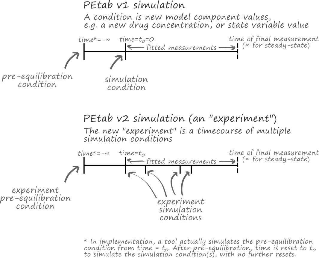
**Figure 3: A comparison of simulations in PEtab v1 and v2.**

Support for math expressions in the condition table (Condition table, Math expressions syntax).
Clarification and specification of various previously underspecified aspects, including overriding values via the condition table (Initialization and parameter application, Detailed semantics).
Support for format extensions.
Observable IDs can now be used in observable and noise formulas (Observable table).
The parameterScale column of the Parameter table is removed. This change was made to simplify the PEtab format. This feature was a constant source of confusion and the interaction with parameter priors was not well-defined. To obtain the same effect, the model parameters can be transformed in the model file.
The initializationPriorType and initializationPriorParameters columns of the Parameter table are removed. Initialization priors are outside the definition of the parameter estimation problem and were a source of confusion.
objectivePriorType and objectivePriorParameters in the Parameter table are renamed to priorDistribution and priorParameters, respectively. This change was made to simplify the PEtab format.
The admissible values for estimate in the Parameter table are now true and false instead of 1 and 0.
Support for new parameter prior distributions in the Parameter table, and clarification that bounds truncate the prior distributions.
The observableTransformation column of the Observable table has been combined with the noiseDistribution column to make its intent clearer. The log10 transformation has been removed, since this was mostly relevant for visualization purposes, and the same effect can be achieved by rescaling the parameters of the respective (natural) log-distributions.
The observableFormula field in the Observable table must not contain any observable IDs. This was previously allowed, but it was not well-defined how to deal with placeholder parameters in this case. The noiseFormula field may contain only the observable ID of the respective observable itself, but no other observable IDs for the same reason.
Placeholders for measurement-specific parameters in observableFormula and noiseFormula are now declared using the observablePlaceholders and noisePlaceholders fields in the Observable table. This replaces the previous observableParameter${n}_${observableId} syntax. The new approach is more explicit and allows for more descriptive and shorter names for the placeholders.
The visualization table has been removed. The PEtab v1 visualization table was not well-defined and not widely used. Visualization is handled by the PEtab Python library which also provides documentation on the respective input format.

Model definition

PEtab 2.0.0 is model format agnostic, meaning it does not depend on a specific model description. The model file is referenced in the PEtab problem description (YAML) by its file name or a URL.

PEtab distinguishes between three types of entities:

Differential entities: Entities that are defined in terms of a time-derivative, e.g., the targets of SBML rate rules or species that change due to participation in reactions (reactants or products).
Algebraic entities: Entities that are defined in terms of algebraic assignments, rather than time derivatives, that are in effect throughout the simulation. They are not necessarily constant, for example, the targets of SBML assignment rules.
Constant entities: Entities are that not differential or algebraic entities. They are defined in terms of an at least piecewise constant value but may be subject to event assignments, e.g., parameters of an SBML model that are not targets of rate rules or assignment rules.

Condition table

The optional condition table defines discrete changes to the simulated model(s). These (sets of) changes typically represent interventions, perturbations, or changes in the environment of the system of interest. These modifications are referred to as (experimental) conditions.

Conditions are applied at specific time points, which are defined in the Experiment table. This allows for the specification of time courses or experiments spanning multiple time periods. A time period is the interval between two consecutive time points in the experiment table (including the first, excluding the second) for a given experiment, or the time between the last time point of an experiment and the end of the simulation (usually, the time point of the last measurement for that experiment in the Measurement table).

The condition table only allows changes in the model state, not the model structure. That means that only constant or differential entities (e.g., constant parameters or model states) can be modified. Algebraic entities (e.g., the targets of SBML assignment rules) cannot be changed.

The condition table is provided as a tab-separated values (TSV) file with the following structure:

conditionId	targetId	targetValue
PETAB_ID	NON_PARAMETER_TABLE_ID	MATH_EXPRESSION
e.g.
conditionId1	modelEntityId1	0.42
conditionId1	modelEntityId2	0.42
conditionId2	modelEntityId1	modelEntityId1 + 3
conditionId2	someSpecies	8
…	…	…

Each row in the condition table represents a single modification to a target entity. The order of rows and columns is arbitrary, but placing conditionId first can enhance readability.

Detailed field description

conditionId [PETAB_ID, REQUIRED]

A unique identifier for the condition associated with the change. This ID is referenced in the Experiment table.
targetId [NON_PARAMETER_TABLE_ID, REQUIRED]

The ID of the entity being modified. The target must be either a constant or differential entity and must not be listed in the Parameter table.
targetValue [MATH_EXPRESSION, REQUIRED]

The value or mathematical expression used to modify the target. When the corresponding condition is applied, the entity specified in targetId is set to the value defined in targetValue (see below for details).

If the model has a concept of species and a species ID is provided, its value is interpreted as either amount or concentration consistent with its usage elsewhere in the model.

Detailed semantics

See Initialization and parameter application for how the changes for the initial period of an experiment are applied and how the model is initialized. For any subsequent time period, the changes defined in the condition table are applied in five consecutive phases:

Evaluation of targetValues

targetValues are first evaluated using the current values of all variables in the respective expressions. The current values are taken from the simulation results at the end of the preceding time period. A special case is simulation time (time), which is set to the start time of the current time period.
Assignment of the evaluated targetValues to their targets

All evaluated targetValues are simultaneously assigned to their respective targets. It is invalid to apply multiple assignments to the same target at the same time.

The interpretation of the assigned value depends on the type of the model and the target entity. For example, for an SBML model and a targetId referring to a species, the targetValue will override the current amount of the species if hasOnlySubstanceUnits=true (amount-based species), or the current concentration if hasOnlySubstanceUnits=false (concentration-based species).

If the target is a compartment, the compartment size is set to the evaluated value of the targetValue expression. The value of a species in such a compartment is not changed by this assignment. I.e., for an amount-based species, the amount of the species will be preserved (the concentration may change accordingly), and for a concentration-based species, the concentration will be preserved (the amount may change accordingly). Mind that this differs from the behavior of an SBML event assignment where compartment size changes always preserve the amounts of species in that compartment.
Update of derived variables

After target values have been assigned, all derived variables (i.e., algebraic entities such as SBML assignment rules or PySB expressions) are updated.
Events and finalization

At this stage, all remaining state- or time-dependent changes encoded in the model are applied, including SBML events. The model state used for the evaluation of trigger functions or the execution of any event assignments (including events with delays) is the model state after (3).

The initial model state for the new period at time = time (Experiment table) is the model state after all these updates have been applied.
Evaluation of observables

If measurements exist for the current timepoint, the observables are evaluated after all changes have been applied. The resulting values are then compared against the corresponding measurements in the measurement table.

Experiment table

The optional experiments table defines a sequence (Figure 3, lower) of experimental conditions (i.e., discrete changes; see Condition table) applied to the model.

The experiment table is provided as a tab-separated values (TSV) file with the following structure:

experimentId	time	conditionId
PETAB_ID	NUMERIC or ‘-inf’	CONDITION_ID
e.g.
timecourse_1	0	condition_1
timecourse_1	10	condition_2
timecourse_1	250	condition_3
patient_3	-inf	condition_1
patient_3	0	condition_2
intervention_effect	-20	no_lockdown
intervention_effect	20	mild_lockdown
intervention_effect	40	severe_lockdown

The order of the rows is arbitrary, but specifying the rows in ascending order of time may improve human readability.

Detailed field description

The experiment table has three mandatory columns experimentId, time, and conditionId:

experimentId [PETAB_ID, REQUIRED]

A unique identifier for the experiment, referenced by the experimentId column in the Measurement table.
time: [NUMERIC or -inf, REQUIRED]

The time at which the specified condition will become active, in the time unit specified in the model. -inf indicates that the respective condition will be simulated until a steady state is reached.

Note

In PEtab, the steady state definition is that all differential entities are at steady state, meaning that all differential entities have reached, and will remain at, a constant value.

Determining whether differential entities are at steady state is left to the simulator and user. Reasonable numerical criteria should be used to determine whether a steady state is reached. Users should share their chosen numerical criteria when sharing their model, for reproducibility.

It can be difficult to determine whether the differential entities are at steady state. For example, events and other discontinuities may occur after an apparent steady state is reached. It is left to the user to avoid situations where this issue is problematic.

If the simulation of a condition with steady state fails to reach a steady state, and the condition is required for the evaluation of simulation at measurement points, the evaluation of the model is not well-defined. In such cases, PEtab interpreters should notify the user, for example, by returning NaN or inf values for the objective function. PEtab does not specify a numerical criterion for steady states. Any event triggers defined in the model must also be checked during this pre-simulation.

Multiple conditions may be applied simultaneously by specifying the same experimentId and time for multiple conditions. The changes associated with these conditions must be disjoint, i.e., no two conditions applied at the same time may involve the same targetId. The union of these changes is applied to the model as if they were specified as a single condition.

time will override any initial time specified in the model, except in the case of time = -ìnf, in which case the model-specified time will be used (or 0, if the model does not explicitly specify an initial time).
conditionId: [PETAB_ID or empty, REQUIRED, REFERENCES(condition.conditionId)]

A reference to a condition ID in the Condition table that will be applied at the given time. If empty, no changes are applied.

For further details, see Detailed semantics.

Measurement table

A tab-separated values files containing all measurements to be used for model training or validation.

Expected to have the following named columns in any (but preferably this) order:

observableId	experimentId	measurement	time
PETAB_ID	PETAB_ID	NUMERIC	NUMERIC\|inf
e.g.
observable1	experiment1	0.42	0
…	…	…	…

(wrapped for readability)

…	[observableParameters]	[noiseParameters]
…	[parameterId\|NUMERIC[;parameterId\|NUMERIC][…]]	[parameterId\|NUMERIC[;parameterId\|NUMERIC][…]]
…
…
…	…	…

Additional (non-standard) columns may be added.

Detailed field description

observableId [PETAB_ID, REQUIRED, REFERENCES(observable.observableId)]

Observable ID as defined in the observable table described below.
experimentId [PETAB_ID or empty, REQUIRED, REFERENCES(experiment.experimentId)]

Experiment ID as defined in the experiment table described below. This column may have empty cells, which are interpreted as use the model as is. This avoids the need for “dummy” conditions and experiments if only a single condition is required. If no experiment is specified, the model simulation is assumed to start at time 0, unless the model specifies a different initial time.
measurement [NUMERIC, REQUIRED]

The measured value in the same units/scale as the model output.
time [NUMERIC OR inf, REQUIRED]

Time point of the measurement in the time unit specified in the employed model, a finite numeric value, or inf (lower-case) for steady-state measurements (the same definition of steady state as in the Experiment table applies here, with the additional sanity check that the steady state occurs during the final experiment period). This value must be greater than or equal to the first time point of the experiment referenced in the experimentId column that is not -inf.

If this time point coincides with the time point of a condition change, the condition change is applied before the observable is evaluated (see Detailed semantics for details).
observableParameters [NUMERIC, STRING OR NULL, OPTIONAL]

Measurement-specific overrides for placeholder parameters in the observableFormula declared in the observable table.

The observable table allows marking some parameters as measurement-specific (see observablePlaceholders there). Their values for a given measurement are specified in this column. The values are separated by semicolons. The order and number of values must match the order and number of placeholders in the observablePlaceholders field of the corresponding observable in the observable table. I.e., if the observable table contains no observable placeholders for the given observable, this field must be empty. The values may be either numeric values or the IDs of parameters from the parameter table.

Different measurements for the same observableId may specify different values. This may be used to account for condition-specific or batch-specific parameters.

If none of the observables referenced in a given measurement table use any noise placeholders, this column may be omitted there.
noiseParameters [NUMERIC, STRING OR NULL, OPTIONAL]

Measurement-specific overrides for placeholder parameters in the noiseFormula declared in the observable table.

The observable table allows marking some parameters as measurement-specific (see noisePlaceholders there). Their values for a given measurement are specified in this column. The values are separated by semicolons. The order and number of values must match the order and number of placeholders in the noisePlaceholders field of the corresponding observable in the observable table. I.e., if the observable table contains no noise placeholders for the given observable, this field must be empty. The values may be either numeric values or the IDs of parameters from the parameter table.

Different measurements for the same observableId may specify different values. This may be used to account for condition-specific or batch-specific parameters.

If none of the observables referenced in a given measurement table use any noise placeholders, this column may be omitted there.
modelId [PETAB_ID, OPTIONAL, REFERENCES(yaml.models.model_id)]

Which model to simulate for each data point. Model IDs are defined by the keys of the models object in the PEtab problem YAML file. This column is required when multiple models are defined in the PEtab problem (see Parameter estimation problems combining multiple models). For problems with a single model, this column is optional, and its values default to the ID of the only model present.

Simulation table

For some applications, it is useful to provide a simulation file that contains the simulation results of the model for the same time points as the measurements. This is useful, for example, for comparing the simulation results with the measurements, or for assessing simulation reproducibility across tools. The simulation table is provided as a tab-separated values (TSV) file with the same structure as the measurement table, only that the measurement column is replaced by the simulation column that contains the simulation results.

Observable table

Parameter estimation requires linking experimental observations to the model of interest. Therefore, one needs to define observables (model outputs) and respective noise models, which represent the measurement process. Since parameter estimation is beyond the scope of SBML, there exists no standard way to specify observables (model outputs) and respective noise models. Therefore, in PEtab observables are specified in a separate table as described in the following. This allows for a clear separation of the observation model and the underlying dynamic model, which allows, in most cases, to reuse any existing SBML model without modifications.

The observable table has the following columns:

observableId	[observableName]	observableFormula
STRING	[STRING]	STRING
e.g.
relativeTotalProtein1	Relative abundance of Protein1	observableParameter1_relativeTotalProtein1 * (protein1 + phospho_protein1 )
…	…	…

(wrapped for readability)

…	noiseFormula	[noiseDistribution]
…	STRING\|NUMBER	see below
…
…	noiseParameter1_relativeTotalProtein1	normal
…	…	…

Detailed field description

observableId [STRING]

Unique identifier for the given observable. Must consist only of upper and lower case letters, digits and underscores, and must not start with a digit. This is referenced by the observableId column in the measurement table.
[observableName] [STRING, OPTIONAL]

Name of the observable. Only used for output, not for identification.
observableFormula [STRING]

Observation function as plain text formula expression. The expression may contain any symbol defined in a model, the mapping table or the parameter table. Often, this is just the ID of a state variable. Furthermore, any parameters introduced through the observablePlaceholders field for the given observable may be used (see below).
observablePlaceholders [LIST[PETAB_ID], OPTIONAL]

A semicolon-separated list of valid PEtab identifiers that have not been introduced elsewhere, marking them as placeholders for measurement-specific parameters. The actual values for these parameters are specified in the observableParameters field of the measurement table. The ordering and number of values in observableParameters must match the ordering and number of placeholders in observablePlaceholders. For an example, see the description of noisePlaceholders below.
noiseFormula [NUMERIC|STRING]

The scale parameter of the noise distribution for the given observable.

Measurement noise can be specified as a numerical value which will default to a Gaussian noise model if not specified differently in noiseDistribution with standard deviation as provided here. In this case, the same standard deviation is assumed for all measurements for the given observable.

Alternatively, some formula expression can be provided to specify more complex noise models. The same rules as for observableFormula apply here. In addition, the current observable ID may be used to refer to the observableFormula expression. In addition to the placeholders declared in observablePlaceholders, placeholders for noise parameters that are declared in noisePlaceholders may be used.
noisePlaceholders [LIST[PETAB_ID], OPTIONAL]

A semicolon-delimited list of valid PEtab identifiers that have not been introduced elsewhere, marking them as placeholders for measurement-specific noise parameters. The actual values for these parameters are specified in the noiseParameters field of the measurement table. The ordering and number of values in noiseParameters must match the ordering and number of placeholders in noisePlaceholders.

For example, a noise model that accounts for measurement-specific relative and absolute contributions for some observable with the ID observable_pErk could be defined as:
```
noise_offset_pErk + noise_scale_pErk * observable_pErk
```
with noise_offset_pErk denoting the absolute and noise_scale_pErk the relative contribution. The corresponding noisePlaceholders would be:
```
noise_offset_pErk;noise_scale_pErk
```
and the noiseParameters in the measurement table could be, for example, 0.1;0.2 resulting in:
```
noise_offset_pErk = 0.1
noise_scale_pErk = 0.2
```
noiseDistribution [STRING, OPTIONAL]

Assumed noise distribution for the measurements of the given observable. The supported noise distributions and the respective interpretation of noiseFormula are given in the table below.

Noise distributions

Denote by $m$ the measured value, $y:=\text{observableFormula}$ the simulated value (the location parameter of the noise distribution), and $\sigma$ the scale parameter of the noise distribution as given via the noiseFormula field (the standard deviation of a normal, or the scale parameter of a Laplace model). Then we have the following effective noise distributions:

Type	`noiseDistribution`	Probability density function (PDF)
Gaussian distribution	`normal`	\[\pi(m\|y,\sigma) = \frac{1}{\sqrt{2\pi}\sigma}\exp\left(-\frac{(m-y)^2}{2\sigma^2}\right)\]
Log-normal distribution (i.e., $\log(m)$ is normally distributed)	`log-normal`	\[\pi(m\|y,\sigma) = \frac{1}{\sqrt{2\pi}\sigma m}\exp\left(-\frac{(\log m - \log y)^2}{2\sigma^2}\right)\]
Laplace distribution	`laplace`	\[\pi(m\|y,\sigma) = \frac{1}{2\sigma}\exp\left(-\frac{\|m-y\|}{\sigma}\right)\]
Log-Laplace distribution (i.e., $\log(m)$ is Laplace distributed)	`log-laplace`	\[\pi(m\|y,\sigma) = \frac{1}{2\sigma m}\exp\left(-\frac{\|\log m - \log y\|}{\sigma}\right)\]

The distributions above are for a single data point. For a collection $D=\{m_i\}_i$ of data points and corresponding simulations $Y=\{y_i\}_i$ and noise parameters $\Sigma=\{\sigma_i\}_i$, the current specification assumes independence, i.e. the full distribution is

\[\pi(D|Y,\Sigma) = \prod_i\pi(m_i|y_i,\sigma_i)\]

Parameter table

A tab-separated value text file containing information on model parameters.

This table must include the following parameters:

Named parameter overrides introduced in targetValue expressions in the condition table, unless already defined in the model
Named parameter overrides introduced in observableParameters or noiseParameters in the measurement table
Parameters introduced in the observableFormula or noiseFormula expressions in the observable table

and must not include:

Placeholder parameters (see observableParameters and noiseParameters above)
Parameters occurring as targetId in the condition table
“Parameters” that are not constant entities (e.g., in an SBML model, the targets of AssignmentRules or EventAssignments)
Any parameters that do not have valid PEtab IDs (e.g., SBML local parameters that are not mapped in the mapping table)

it may include:

Any model parameter that was not excluded above

One row per parameter with arbitrary order of rows and columns:

parameterId	[parameterName]	lowerBound	upperBound	nominalValue	estimate	…
PETAB_ID	[STRING]	NUMERIC	NUMERIC	NUMERIC	true\|false	…
k1		1e-5	1e5	100	true	…
…	…	…	…	…	…	…

(wrapped for readability)

…	[priorDistribution]	[priorParameters]
…	see below	see below
…	normal	1000;100
…	…	…

Additional columns may be added.

See Initialization and parameter application for details on how and when the values of parameter table parameters are applied.

Detailed field description

parameterId [PETAB_ID, REQUIRED]

The parameterId of the parameter described in this row. This has to match the ID of a parameter specified in at least one model, a parameter introduced as override in the condition table, or a parameter occurring in the observableParameters or noiseParameters column of the measurement table (see above).
parameterName [STRING, OPTIONAL]

Parameter name to be used e.g. for plotting etc. Can be chosen freely. May or may not coincide with the SBML parameter name.
lowerBound [NUMERIC]

Lower bound of the parameter used for estimation. Optional, if estimate==false.
upperBound [NUMERIC]

Upper bound of the parameter used for estimation. Optional, if estimate==false.
nominalValue [NUMERIC]

Some parameter value to be used if the parameter is not subject to estimation (see estimate below). Optional, unless estimate==false.
estimate [true | false]

true or false (case-sensitive), depending on, if the parameter is estimated (true) or set to a fixed value (false) (see nominalValue).
priorDistribution [STRING, OPTIONAL]

Prior types used for the MAP objective function and for Bayesian inference. It is valid to have no priors. However, if priors are specified for a subset of parameters, this defaults to the uniform prior (with priorParameters set to lowerBound;upperBound) for the other parameters.

Prior distributions are truncated by the lowerBound and upperBound if the prior’s domain exceeds the parameter bounds. A non-truncated prior can be created by setting the parameter bounds to match the prior’s domain (e.g., 0 and inf for log-normal). For supported prior distributions see prior distributions.
priorParameters [STRING, OPTIONAL]

Prior parameters used for the MAP objective function and for Bayesian inference. priorParameters is required if priorDistribution is non-empty.

Only numeric values are supported (no parameter IDs). For available parameters see prior distributions.

Prior distributions

The prior distributions supported for the MAP objective function and for Bayesian inference are listed below. PEtab only supports univariate prior distributions. The probability density functions (PDFs) below assume that the parameter bounds are wide enough to not truncate the distributions. If the parameter bounds are narrower than the distribution’s support, the distributions are truncated, resulting in the following truncated prior distribution:

\[\pi_{\text{trunc}}(x) = \frac{\pi(x)}{\text{CDF}(\text{upperBound}) - \text{CDF}(\text{lowerBound})}\]

where $\pi(x)$ is the PDF of the non-truncated distribution and $\text{CDF}(\cdot)$ its cumulative distribution function.

Let $x$ denote the parameter value and $\Gamma$ the Gamma function., then the following prior distributions are supported:

`priorDistribution`	`priorParameters`	Probability density function (PDF)	Domain
`cauchy`	location ($\mu$); scale ($\sigma$)	\[\pi(x\|\mu, \sigma) = \frac{1}{\pi \sigma \left( 1 + \left(\frac{x - \mu}{\sigma} \right)^2\right)}\]	$(-\infty, \infty)$
`chisquare`	degrees of freedom ($\nu$)	\[\pi(x\|\nu) = \frac{x^{\nu/2-1}e^{-x/2}}{2^{\nu/2}\Gamma(\nu/2)}\]	$(0, \infty)$
`exponential`	scale ($\theta$)	\[\pi(x\|\theta) = \frac{1}{\theta}e^{-x/\theta}\]	$(0, \infty)$
`gamma`	shape ($\alpha$); scale ($\theta$)	\[\pi(x\|\alpha, \theta) = \frac{x^{\alpha - 1}e^{-x/\theta}}{\Gamma(\alpha)\theta^{\alpha}}\]	$(-\infty, \infty)$
`laplace`	location ($\mu$); scale ($\sigma$)	\[\pi(x\|\mu, \sigma) = \frac{1}{2\sigma}\exp\left(- \frac{\|x - \mu \|}{\sigma}\right)\]	$(-\infty, \infty)$
`log-laplace`	location ($\mu$); scale ($\sigma$)	\[\pi(x\|\mu, \sigma) = \frac{1}{2\sigma x} \exp\left( - \frac{\|\log(x) - \mu\|}{\sigma} \right)\]	$(0, \infty)$
`log-normal`	mean ($\mu$); standard deviation ($\sigma$)	\[\pi(x\|\mu, \sigma) = \frac{1}{x \sqrt{2\pi}\sigma} \exp\left(- \frac{\left(\log(x) - \mu\right)^2}{2\sigma^2}\right)\]	$(0, \infty)$
`log-uniform`	lower bound ($a$); upper bound ($b$)	\[\pi(x\|a, b) = \frac{1}{x\left( \log(b) - \log(a) \right)}\]	$[a, b]$
`normal`	mean ($\mu$); standard deviation ($\sigma$)	\[\pi(x\|\mu,\sigma) = \frac{1}{\sqrt{2\pi}\sigma}\exp\left(-\frac{(x-\mu)^2}{2\sigma^2}\right)\]	$(-\infty, \infty)$
`rayleigh`	scale ($\sigma$)	\[\pi(x\|\sigma) = \frac{x}{\sigma^2}\exp\left(\frac{-x^2}{2\sigma^2}\right)\]	$(0, \infty)$
`uniform`	lower bound ($a$); upper bound ($b$)	\[\pi(x\|a, b) = \frac{1}{b - a}\]	$[a, b]$

Mapping table

The mapping table maps PEtab entity IDs to model entity IDs, and may be used for additional annotations of model or PEtab entities. This file is optional.

This file may be used to provide PEtab-compatible aliases to model entities whose ID in the model would not be a valid identifier in PEtab (e.g., due to inclusion of blanks, dots, or other special characters), and thus, would not be allowed in the PEtab problem files.

The TSV file has two mandatory columns, petabEntityId and modelEntityId. Additional columns are allowed.

petabEntityId	modelEntityId	[name]
PETAB_ID	STRING	STRING
reaction1_k1	reaction1.k1	reaction1 k1

Detailed field description

petabEntityId [PETAB_ID, REQUIRED]

A valid PEtab identifier (see Identifiers) that is not defined in any other part of the PEtab problem. This identifier may be referenced in condition, measurement, parameter and observable tables, but cannot be referenced in the model itself.

The petabEntityId may be the same as the modelEntityId, but it must not be used to alias an entity that already has a valid PEtab identifier. This restriction is to avoid unnecessary complexity in the PEtab problem files.
modelEntityId [STRING or empty, REQUIRED]

A globally unique identifier defined in any model, or empty if the entity is not present in any model. This does not have to be a valid PEtab identifier. Rows with empty modelEntityId serve as annotations only.

For example, in SBML, local parameters may be referenced as $reactionId.$localParameterId, which are not valid PEtab IDs as they contain a . character. Similarly, this table may be used to reference specific species in a BNGL model that may contain many unsupported characters such as ,, ( or .. However, please note that IDs must exactly match the species names in the BNGL-generated network file, and no pattern matching will be performed.
name [STRING or empty, OPTIONAL]

A human-readable name for the entity. This is optional and may be used for reporting or visualization purposes. Any tool making use of this value should default to the petabEntityId if this field is empty.

YAML file for grouping files

To link the model, measurement table, condition table, etc. in an unambiguous way, we use a YAML file.

This file also allows specifying a PEtab version and employed PEtab extensions.

Furthermore, this can be used to describe parameter estimation problems comprising multiple models (more details below).

The format is described in the jsonschema, which allows for easy validation:

# For syntax see: https://json-schema.org/understanding-json-schema
$schema: "https://json-schema.org/draft/2020-12/schema"
description: PEtab parameter estimation problem config file schema

properties:

  format_version:
    anyOf:
      - type: string
        #  (corresponding to PEP 440).
        pattern: ^([1-9][0-9]*!)?(0|[1-9][0-9]*)(\.(0|[1-9][0-9]*))*((a|b|rc)(0|[1-9][0-9]*))?(\.post(0|[1-9][0-9]*))?(\.dev(0|[1-9][0-9]*))?$
      - type: integer

    description: Version of the PEtab format

  id:
    type: string
    description: |
      Identifier of the PEtab problem.

      This is optional and has no effect on the PEtab problem itself.
    pattern: "^[a-zA-Z_]\\w*$"

  parameter_files:
    type: array
    description: |
      List of PEtab parameter files.

    items:
        type: string
        description: |
          File name (absolute or relative) or URL to a PEtab parameter table.

  model_files:
    type: object
    description: One or multiple models

    # the model ID
    patternProperties:
      "^[a-zA-Z_]\\w*$":
        type: object
        properties:
          location:
            type: string
            description: Model file name or URL
          language:
            type: string
            description: |
              Model language, e.g., 'sbml', 'cellml', 'bngl', 'pysb'
        required:
          - location
          - language
    additionalProperties: false

  measurement_files:
    type: array
    description: List of PEtab measurement files.

    items:
      type: string
      description: PEtab measurement file name or URL.

  condition_files:
    type: array
    description: List of PEtab condition files.

    items:
      type: string
      description: PEtab condition file name or URL.

  experiment_files:
    type: array
    description: List of PEtab experiment files

    items:
      type: string
      description: PEtab experiment file name or URL.

  observable_files:
    type: array
    description: List of PEtab observable files.

    items:
      type: string
      description: PEtab observable file name or URL.

  mapping_files:
    type: array
    description: List of PEtab mapping files.

    items:
      type: string
      description: PEtab mapping file name or URL.

  extensions:
    type: object
    description: |
      PEtab extensions being used.
    patternProperties:
      "^[a-zA-Z][\\-\\w]*$":

        type: object
        description: |
          Information on a specific extension
        properties:
          version:
            type: string
            pattern: ^([1-9][0-9]*!)?(0|[1-9][0-9]*)(\.(0|[1-9][0-9]*))*((a|b|rc)(0|[1-9][0-9]*))?(\.post(0|[1-9][0-9]*))?(\.dev(0|[1-9][0-9]*))?$
          required:
            type: boolean
            description: |
              Indicates whether the extension is required for the
              mathematical interpretation of the problem.
        required:
          - version
          - required
      additionalProperties: true

    additionalProperties: false

required:
  - format_version
  - parameter_files
  - model_files
  - observable_files
  - measurement_files

additionalProperties: false

Parameter estimation problems combining multiple models

Purpose

PEtab supports defining multiple models within a single problem specification. This feature is designed to enable users to define experiment-specific model variants or submodels. Rather than implementing a single global, parameterized model, users can define multiple smaller, self-contained models that differ structurally as needed.

This approach offers several benefits:

Simplified model definition for users, as each variant can be independently specified.
Improved simulation performance for tool developers, as smaller models can be simulated more efficiently.

Scope and Application

While multiple models are intended to be applied to different experiments, model selection is specified at the level of individual data points in the Measurement table. This design enables:

Reuse of experiments across models.
Fine-grained model-to-data assignment.

With the exception of the Measurement table, all other PEtab tables apply to all models. Parameters listed in the parameter table are defined globally and shared across all models. In contrast, entries in all other tables implicitly define model-specific instances of observables, conditions, experiments, etc., with their respective PEtab IDs existing in local, model-specific namespaces. Each PEtab subproblem defined in this way must constitute a valid PEtab problem on its own.

This design has several implications:

A single experiment may need to be simulated with different models for different measurements. However, a single simulation of a given experiment is always performed using one single model.
Each model may be associated with a distinct subset of experiments.
The number of conditions to be simulated for a model-specific instance of an experiment may vary across models.
Each parameter defined in the Parameter table has a shared value across all models. Parameters not listed in the parameter table do not share values, which can result in model-specific instantiations of model observables referencing these parameters.

Validation Rules

For any given model, only those experiments and observables that appear in the same rows of the Measurement table need to be valid. This means that all symbols used in the corresponding observableFormula and all symbols assigned in the associated condition definitions must be defined in the model.

Conditions and observables that are not applied to a model do not need to be valid for that model.

Initialization and parameter application

The following describes how the model is initialized and how other PEtab parameter values are applied before the simulation starts. This procedure is executed for each model and experiment combination defined in the PEtab problem.

Pre-initialization
1. Parameters values for parameters that occur in the parameter table are applied to the uninitialized model. Uninitialized means that no model-internal initial values have been computed yet (e.g., in SBML models, no initial assignments have been evaluated and no derived initial quantities such as concentrations have been computed yet). For estimated parameters, the respective externally-provided values are applied and for non-estimated parameters, the nominal values from the parameter table are applied.
2. The time is set to the start time of the first period of the given experiment (or 0 if there is no explicit experiment), and any experiment-specific conditions provided for the first period are applied (see Detailed semantics for details). Target value expressions for the first period must not refer to model entities that are not also listed in the parameter table.
This pre-initialization replaces any model-internal initial values (or initialization constructs such as SBML’s initialAssignments) that would alter the initial time, the values of the parameters contained in the parameter table or any target values from the condition table.
Model initialization

The model is initialized according to the model semantics, e.g., by evaluating the initial assignments or applying the initial values of state variables.
Simulation

Model simulation starts with evaluating any event triggers at the initial time, applying pending event assignments, and evaluating the observables at the initial time (Steps 4 and 5 in Detailed semantics).

For any subsequent experiment periods, the steps described in Detailed semantics are applied at their start times.

Frequentist vs. Bayesian inference

PEtab supports maximum likelihood estimation, maximum a posteriori (MAP) estimation, and Bayesian inference.

For MAP estimation and Bayesian inference, the prior distributions $p(\theta)$ of the model parameters $\theta$ are specified in the parameter table (priorDistribution and priorParameters columns, as described above), while for maximum likelihood estimation, the prior distributions are not specified. If priors are only specified for a subset of inferred parameters, the remaining parameters are assumed to have a uniform prior between their lower and upper bounds.

For maximum likelihood estimation, the objective function is the negative log-likelihood of the data given the model $\mathcal{M}$ with parameters :

\[ \begin{align}\begin{aligned}\mathcal{L}_{\text{ML}}(\theta) = - \log p(\mathcal{D} \mid \mathcal{M}, \theta)\\\theta_{\text{ML}} = \arg\min_{\theta} \mathcal{L}_{\text{ML}}(\theta)\end{aligned}\end{align} \]

Where $p(\mathcal{D} \mid \mathcal{M}, \theta)$ is the likelihood as described under Noise distributions.

For MAP estimation, the objective function is the unnormalized negative log-posterior of the data given the model and the parameters:

\[ \begin{align}\begin{aligned}\mathcal{L}_{\text{MAP}}(\theta) = - \log p(\mathcal{D} \mid \mathcal{M}, \theta) - \log p(\theta)\\\theta_{\text{MAP}} = \arg\min_{\theta} \mathcal{L}_{\text{MAP}}(\theta)\end{aligned}\end{align} \]

Different tools may use different objective function formulations internally, as long as they preserve the optima. However, tools should provide the final objective function value, as the negative log-likelihood or unnormalized negative log-posterior, to facilitate comparison and reproducibility.

Example

In the case of independently and normally distributed noise, the negative log-likelihood would be:

\[\mathcal{L}_{\text{ML}}(\theta) = \frac{1}{2} \sum_{i=1}^N \left( \log(2\pi \sigma_i^2) + \frac{(m_i - y_i)^2}{\sigma_i^2} \right)\]

where $m_i$ is the measurement, $y_i$ is the model output, and $\sigma_i$ is the standard deviation of the noise for the $i$-th measurement.

Math expressions syntax

This section describes the syntax of math expressions used in PEtab files, such as the observable formulas.

Supported symbols, literals, and operations are described in the following. Whitespace is ignored in math expressions.

Symbols

The supported identifiers are:
- parameter IDs from the parameter table
- model entity IDs that are globally unique and have a clear interpretation in a math expression context
- observable IDs from the observable table
- PEtab placeholder IDs in the observable and noise formulas
- PEtab entity IDs in the mapping table
- time for the model time
- PEtab function names listed below

Identifiers are not supported if they do not match the PEtab identifier format. PEtab expressions may have further context-specific restrictions on supported identifiers.

The functions defined in PEtab are tabulated below. Other functions, including those defined in the model, remain undefined in PEtab expressions.
Special symbols (such as $e$ and $\pi$) are not supported, and neither is NaN (not-a-number).

Model time

The model time is represented by the symbol time, which is the current simulated time, not the current duration of simulated time; if the simulation starts at $t_0 \neq 0$, then time is not the time since $t_0$.

Literals

Numbers

All numbers, including integers, are treated as floating point numbers of undefined precision (although no less than double precision should be used. Only decimal notation is supported. Scientific notation is supported, with the exponent indicated by e or E. The decimal separator is indicated by .. Examples of valid numbers are: 1, 1.0, -1.0, 1.0e-3, 1.0e3, 1e+3. The general syntax in PCRE2 regex is \d*(\.\d+)?([eE][-+]?\d+)?. inf and -inf are supported as positive and negative infinity.

Booleans

Boolean literals are true and false.

Operations

Operators

The supported operators are:

Supported operators in PEtab math expressions.
Operator	Precedence	Interpretation	Associativity	Arguments	Evaluates to
`f(arg1[, arg2, ...])`	1	call to function f with arguments arg1, arg2, …	left-to-right	any	input-dependent
`()`	1	parentheses for grouping acts like identity		any single expression	argument
`^`	2	exponentiation (shorthand for pow)	right-to-left	float, float	float
`+` `-`	3	unary plus unary minus	right-to-left	float	float
`!`	3	not		bool	bool
`*` `/`	4	multiplication division	left-to-right	float, float	float
`+` `-`	5	binary plus, addition binary minus, subtraction	left-to-right	float, float	float
`<` `<=` `>` `>=`	6	less than less than or equal to greater than greater than or equal to	left-to-right	float, float	bool
`==` `!=`	6	is equal to is not equal to	left-to-right	(float, float) or (bool, bool)	bool
`&&` `\|\|`	7	logical and logical or	left-to-right	bool, bool	bool
`,`	8	function argument separator	left-to-right	any

Note that operator precedence might be unexpected, compared to other programming languages. Use parentheses to enforce the desired order of operations.

Operators must be specified; there are no implicit operators. For example, a b is invalid, unlike a * b.

Functions

The following functions are supported:

Supported functions
Function	Comment	Argument types	Evaluates to
`pow(a, b)`	power function b-th power of a	float, float	float
`exp(x)`	exponential function pow(e, x) (e itself not a supported symbol, but `exp(1)` can be used instead)	float	float
`sqrt(x)`	square root of `x` `pow(x, 0.5)`	float	float
`log(a, b)` `log(x)` `ln(x)` `log2(x)` `log10(x)`	logarithm of `a` with base `b` `log(x, e)` `log(x, e)` `log(x, 2)` `log(x, 10)` (`log(0)` is defined as `-inf`) (NOTE: `log` without explicit base is `ln`, not `log10`)	float[, float]	float
`sin` `cos` `tan` `cot` `sec` `csc`	trigonometric functions	float	float
`arcsin` `arccos` `arctan` `arccot` `arcsec` `arccsc`	inverse trigonometric functions	float	float
`sinh` `cosh` `tanh` `coth` `sech` `csch`	hyperbolic functions	float	float
`arcsinh` `arccosh` `arctanh` `arccoth` `arcsech` `arccsch`	inverse hyperbolic functions	float	float
`piecewise(` `true_value_1,` `condition_1,` `[true_value_2,` `condition_2,]` `[...]` `[true_value_n,` `condition_n,]` `otherwise` `)`	The function value is the `true_value` for the first `true` `condition` or `otherwise` if all conditions are `false`.	`value`: all float or all bool `condition*`: all bool	float
`abs(x)`	absolute value `piecewise(x, x>=0, -x)`	float	float
`sign(x)`	sign of `x` `piecewise(1, x > 0, -1, x < 0, 0)`	float	float
`min(a, b)` `max(a, b)`	minimum / maximum of {`a`, `b`} `piecewise(a, a<=b, b)` `piecewise(a, a>=b, b)`	float, float	float

Boolean ↔ float conversion

Boolean and float values are implicitly convertible. The following rules apply:

bool → float: true is converted to 1.0, false is converted to 0.0.

float → bool: 0.0 is converted to false, all other values are converted to true.

Operands and function arguments are implicitly converted as needed. If there is no signature compatible with the given types, Boolean values are promoted to float. If there is still no compatible signature, float values are demoted to boolean values. For example, in 1 + true, true is promoted to 1.0 and the expression is interpreted as 1.0 + 1.0 = 2.0, whereas in 1 && true, 1 is demoted to true and the expression is interpreted as true && true = true.

Identifiers

All identifiers in PEtab may only contain upper and lower case letters, digits and underscores, and must not start with a digit. In PCRE2 regex, they must match [a-zA-Z_][a-zA-Z_\d]*.
Identifiers are case-sensitive.
Identifiers must not be a reserved keyword (see below).
Identifiers must be globally unique within the PEtab problem. PEtab does not put any further restrictions on the use of identifiers within the model, which means modelers could potentially use model-format–specific (e.g. SBML) function names as identifiers. However, this is strongly discouraged.

Reserved keywords

The following keywords, case-insensitive, are reserved and must not be used as identifiers:

true, false: Boolean literals, used in PEtab expressions.
inf: Infinity, used in PEtab expressions and for steady-state measurements
time: Model time, used in PEtab expressions.
nan: Undefined in PEtab, but reserved to avoid implementation issues.
PEtab math function names (Functions)

`priorDistribution`	`priorParameters`	Probability density function (PDF)	Domain
`cauchy`	location (\(\mu\)); scale (\(\sigma\))	\[\pi(x\|\mu, \sigma) = \frac{1}{\pi \sigma \left( 1 + \left(\frac{x - \mu}{\sigma} \right)^2\right)}\]	\((-\infty, \infty)\)
`chisquare`	degrees of freedom (\(\nu\))	\[\pi(x\|\nu) = \frac{x^{\nu/2-1}e^{-x/2}}{2^{\nu/2}\Gamma(\nu/2)}\]	\((0, \infty)\)
`exponential`	scale (\(\theta\))	\[\pi(x\|\theta) = \frac{1}{\theta}e^{-x/\theta}\]	\((0, \infty)\)
`gamma`	shape (\(\alpha\)); scale (\(\theta\))	\[\pi(x\|\alpha, \theta) = \frac{x^{\alpha - 1}e^{-x/\theta}}{\Gamma(\alpha)\theta^{\alpha}}\]	\((-\infty, \infty)\)
`laplace`	location (\(\mu\)); scale (\(\sigma\))	\[\pi(x\|\mu, \sigma) = \frac{1}{2\sigma}\exp\left(- \frac{\|x - \mu \|}{\sigma}\right)\]	\((-\infty, \infty)\)
`log-laplace`	location (\(\mu\)); scale (\(\sigma\))	\[\pi(x\|\mu, \sigma) = \frac{1}{2\sigma x} \exp\left( - \frac{\|\log(x) - \mu\|}{\sigma} \right)\]	\((0, \infty)\)
`log-normal`	mean (\(\mu\)); standard deviation (\(\sigma\))	\[\pi(x\|\mu, \sigma) = \frac{1}{x \sqrt{2\pi}\sigma} \exp\left(- \frac{\left(\log(x) - \mu\right)^2}{2\sigma^2}\right)\]	\((0, \infty)\)
`log-uniform`	lower bound (\(a\)); upper bound (\(b\))	\[\pi(x\|a, b) = \frac{1}{x\left( \log(b) - \log(a) \right)}\]	\([a, b]\)
`normal`	mean (\(\mu\)); standard deviation (\(\sigma\))	\[\pi(x\|\mu,\sigma) = \frac{1}{\sqrt{2\pi}\sigma}\exp\left(-\frac{(x-\mu)^2}{2\sigma^2}\right)\]	\((-\infty, \infty)\)
`rayleigh`	scale (\(\sigma\))	\[\pi(x\|\sigma) = \frac{x}{\sigma^2}\exp\left(\frac{-x^2}{2\sigma^2}\right)\]	\((0, \infty)\)
`uniform`	lower bound (\(a\)); upper bound (\(b\))	\[\pi(x\|a, b) = \frac{1}{b - a}\]	\([a, b]\)